An Adventure with Excel

I have a rather old-fashioned attitude to spreadsheet applications - I tend to use them to do maths on columns of numbers and plot graphs and that's about it.  That's what they were invented for, after all.  Within the last year I have used conditional formatting to highlight certain cells that are important, and more recently a work colleague used it to identify chemicals in a spreadsheet of our stock which need to have a COSHH assessment or a COSHH assessment plus an exposure record, based on the hazard codes listed for each of the chemicals.  That worked very well, but my lazy nerd brain started to think that there must be a way to do this that didn't involve laboriously typing a conditional formatting rule for each and every triggering hazard code.  Wasn't there some way that a range of cells could be used to store the hazard codes for COSHH triggers and another one to store the hazard codes that require an exposure record to be kept and use a formula that says "if that cell contains any of those codes then you need a COSHH assessment (or that plus an exposure record)".  That way, you'd be able to simply replicate that formula down a column so it will work on every chemical in the list, and use only 2 conditional formatting rules (do we need COSHH?, do we need an exposure record?) to decide what colour to make the cell.  You'd also have a value in a cell that could be used to trigger some other action somewhere else in the spreadsheet if you need it.

This turned out to be rather more complex a problem than I'd anticipated.  "Do any of these search terms occur in the text in that cell" turns out to be a harder question to answer than it looks because Excel doesn't have a function to answer it directly.  What it does have is more complex and versatile, but that means some extra processing of the search results are required to get what you want.

A Note About Boolean Functions in Excel.

Boolean functions are those which return a value of true or false.  Computers use numbers to represent those values.  In Excel, true is represented by the number 1, and false by zero.  You can force Excel to show you the numeric value by preceding a boolean function with two dashes "--".  Open a blank worksheet and put the following into a cell:  "=(1=1)"  without the quotes.  That might look odd if you're not used to this sort of thing, what it means is " true or false, 1=1?".  I hope it's obvious that one does equal one and that this is therefore true.  When you press 'return', Excel should confirm this by displaying 'TRUE' in the cell you typed the formula into.  Into the cell below, put this: "=(1=2)".  That should display 'FALSE'.

Now try putting two dashes in front of the expressions you used before,  e.g. "=--(1=1)".  You should now see "1" for the true expression and "0" for the false one.  Since these have numerical values, you can do calculations with them, in fact, you can get the same result as using the two dashes by multiplying by 1 the result of a boolean expression, i.e. instead of "=--(1=1)" you can  use "=(1=1)*1".  Try it, it does work. It's also a trick often used in programming languages to perform a calculation only if a condition is satisfied - if the condition is false then the calculation gets multiplied by zero, and the result is therefore zero, if the condition is true then the calculation has the result 

expected.

One final thing before moving on:  What if we want to test if the outcome of some other function is true or false?  do we need it to be explicitly "1" or "0"?  what if it is some other number?  what if it's a text string?  or blank?  Excel will interpret any non-zero number as TRUE.  Any non-zero number - it could be negative, or fractional, it doesn't matter.  If it's a number and it's not exactly equal to zero, then as far as boolean logic is concerned, it's TRUE.  Zero is FALSE, obviously, and so is a blank cell.  Text strings will generate an error (#VALUE! will be displayed).

Back to the Problem

A quick recap:  we want to find out if a particular cell containing a string of text (all the hazard codes for a particular chemical) contains any one of a series of shorter strings of text (the codes that trigger an exposure record and/or a COSHH assessment).   Here is a link to a workbook I created to explore this problem and demonstrate the solution.  Download it to try out the exercises below.

This is the formula which will return TRUE if any of the codes is found in the cell that is searched.

=(SUMPRODUCT(--ISNUMBER(SEARCH(<range containing search terms>,cell to be searched)))>0)

That's a lot of nested brackets, so before breaking it down into simpler parts, let's just note that the outer brackets basically say (something >0) which makes the whole thing a boolean expression, which will return TRUE if something is greater than zero, FALSE otherwise.

The SEARCH Function

SEARCH(<range containing search terms>,cell to be searched).  This is not case-sensitive.  If you ever need to do a similar thing, but with a case-sensitive search, the similar FIND function is what you want.

If you look at the workbook linked to earlier, cell J3 contains a formula like the above, only with actual cell references instead of descriptors.  It says the search terms are in the range of cells from $H$3 to $I$7.  The $ signs mean that these are absolute references, i.e. if the formula is copied elsewhere, they will not be updated because the formula has moved - the same cells will still be used for the search terms.  The cell to be searched is B3.  That's a relative cell reference - that will be updated if the formula is copied elsewhere.  If we were only checking for one search term, i.e. <range containing search terms> is just one cell, then this would return only one result.  If the search term were found, it would return the position within the cell being searched where the found search term began. If it is not found, then an error is returned. Because we have searched for a range of terms, we get an array of results, one for each search term.  You can see in the workbook that Excel has helpfully spilled out the results into the surrounding cells so that we can see them.  Those which say "#VALUE!" are those which did not contain the search term, those with a number did find the search term.  J3 contains the result of searching for "code01" - it's the first thing in cell B3 so starts in position 1.  K4 is the result of searching for "code07" - it begins with the 25th character in cell B3. 

This is all very well, but we just want one answer - were any codes found or not?  to do that, we need to count the number of codes found, and see if it is greater than one.

Is it a Number?

=(SUMPRODUCT(--ISNUMBER(SEARCH(<range containing search terms>,cell to be searched)))>0)

When the SEARCH function finds one of the codes, the result is a number, otherwise not a number.  the ISNUMBER function will return TRUE if its argument is a number, FALSE otherwise.  So if we modify the function in cell J3 by wrapping ISNUMBER() around it:

=ISNUMBER(SEARCH($H$3:$I$7,B3))  the array of cells containing the SEARCH results will display TRUE or FALSE instead.  Then if we prefix that with "--" we will get zeroes and ones instead.

Count 'Em Up

That brings us to the final and most complex part of our formula:  the SUMPRODUCT function.  This will multiply corresponding elements of multiple arrays and add the results together to give one number.  With only one array, such as we have - the array of results from our SEARCH, you simply get the sum of the elements.  After we have applied --ISNUMBER to the array, the elements will be either 1 (if a code was found) or zero.  The result of applying SUMPRODUCT() to our formula will therefore be the number of codes found - if that's greater than zero, then a code has been found.

Just a COSHH? or Do We Need and Exposure Record Too?

You remember that we can do calculations with the result of a boolean function?  Well, we can do that here.  If we use two versions of the formula, one which will search for COSHH triggers (the codes in cells H3-H7) and multiply the result by 1, the other will search for exposure record triggers (the codes in cells I3-I7) and multiply the result by 10, then add those together, we can distinguish between those chemicals which don't need a COSHH assessment (result will be 0), those which need only a COSHH assessment (result will be 1) and those which also need an exposure record (result will be 10 or 11).  Such a formula can be found in cells E3 to E7.  It's rather long and looks like this:

=(SUMPRODUCT(--ISNUMBER(SEARCH($H$3:$H$7,B3)))>0)*1  +  

  (SUMPRODUCT(--ISNUMBER(SEARCH($I$3:$I$7,B3)))>0)*10

Adding Some Colour

Now, at last, we can get back to some conditional formatting to colour code the cells with the hazard codes for each chemical, i.e. B3 to B7.  I have chosen yellow to indicate that a COSHH assessment is required, red to indicate that an exposure record is also required.  That range of cells has two conditional formatting rules applied to it, both based on a formula.

$E1>=1   sets the fill colour to yellow

$E1>=10 sets the fill colour to red

Note the the cell reference in both is mixed:  the column reference is absolute ($E), the row reference is relative (1).  This is so that it will be updated before checking, i.e. the formula will always look at column E, but will adjust for the row, so the formatting for, e.g, B5 will look at the value in E5.

Hope that helps somebody!

Further Notes

Rather than using the codified results in E3 to E7, we could work out directly whether a COSHH assessment or COSHH plus exposure record is needed using formulas in columns C and D.  For column D (exposure record needed) we could simply put iinto D3:

=IF((SUMPRODUCT(--ISNUMBER(SEARCH($I$3:$I$7,B3)))>0),"Yes","")

.. and fill down for the rest of that column.

For column C, it's a bit more complex because if an exposure record is needed, then a COSHH assessment is also needed.  We could simply include all the exposure record triggers in the block of COSHH triggers as well as having them separate, or do something like this for C3 and fill down.

=IF(OR(SUMPRODUCT(--ISNUMBER(SEARCH($I$3:$I$7,B3)))>0),SUMPRODUCT(--ISNUMBER(SEARCH($H$3:$H$7,B3))),"Yes","")

which will work but that formula is getting very long-winded.  A simpler approach might be to expand the range of codes to check for COSHH triggers so that it includes the exposure record trigers also, i.e. search the range $H$3 to $I$7.  There's a big pitfall waiting for anyone who does that, though, and it opens up as soon as there are more COSHH triggers than exposure record triggers (which there are in reality).

Try this exercise: take the formula given above for D3, put that into cell D3 and copy down to D7.  That won't change the results at all, showing that the formula works

Now put this formula into C3 and copy down to D7.  It will expand the search to cover columns H and I:

=IF((SUMPRODUCT(--ISNUMBER(SEARCH($H$3:$I$7,B3)))>0),"Yes","")

Again there will be no change to the results, because the number of codes in each column is the same.  

Check that cell J3 still contains the search formula: =SEARCH($H$3:$I$7,B3) and delete the contents of cell I7, leaving it blank.  Now, apparently, everything needs a COSHH assessment and an exposure record.  What's happened?  If you look at cell K7, you'll see that it contains "1", which would mean that it has found the contents of the blank cell I7.  This will always happen if you search for 'nothing' in Excel, since anything contains 'nothing - plus something else'.  I assume that's the logic of this anyway.  It seems more logical to me that 'nothing' would be found at position zero rather than position 1,but that would not help us with this one - zero is still a number and would be detected by ISNUMBER()

There are some simple workarounds - firstly, use the more complex expression above, and just search the areas with values in them.  Secondly, use an innocuous value for the 'empty' cells - put something like '####' (which should never show up in a real hazard code) in I7 and the problem goes away.

Replacing 3D Printer Controller Board.

New board adapter shown in place.

I chose to replace the controller board in my Copymaster 300 again.  This had already been upgraded to a 32-bit board (Bigtreetech SKR v1.3 with TMC2208 stepper drivers)  when the original controller failed.  There wasn't anything wrong with it this time, in fact it was working well, so why change it?  Because I'm a cheapskate, that's why.  There's a little more to it than that though.  I found a frame in a metal skip that I thought would be a good basis for a 3d printer, so I needed a controller board for it and ordered an SKR Mini E3 with a set of integrated TMC2209 drivers.  This is a more compact board than the SKR V1.3 and has all the features that the Copymaster needs, plus it should run cooler in the confined space of the Copymaster's controller box.  It seemed a good plan to use it for the Copymaster and retrieve the SKR V1.3 for the new project.  To that end, I designed another adapter to fit the board into the case using the mounting points for the original board.


There was just one real concern, and that was the MOSFET controlling current to the bed heater.  The SKR mini E3 was designed to work with a Creality Ender 3, which has a smaller build bed and therefore a less powerful heater.

MOSFETs and Power Dissipation

Board mounted on adapter showing underside

Board mounted on adapter showing top side

The heated bed has a cold resistance of 2.5Ω and is designed to work from 24V.  It will therefore draw about 10A of current.  The SKR Mini uses a VS3060AD mosfet, which has an on-state resistance of 15mΩ when conducting 10A (worst case).  That gives a power dissipation of 10x10x0.015 = 1.5W.  That's well within its rated power dissipation but I wouldn't like to ask it to do that without some extra heat sinking.  So I added some, in the form of a short length of heatsink over the top of it and also the hot-end mosfet, plus another strip of heatsink over the pads provided on the underside of the board.  I also added a longer strip to cover the pads beneath the stepper drivers, which will get some airflow from the case fan when installed.  In fact, given that the mosfets & stepper drivers are designed to shed most of their waste heat through the circuit board they are mounted on, these heatsinks underneath the board probably shed heat better than those little blue ones on top of the drivers. 

I couldn't find any sensible information about the Ender 3's bed resistance, power or current draw, but assuming it's going to be about the same as my Mendel, which has a similar bed size, 100W seems about right, which would give a current draw of about 4A since the Ender 3 also works on 24V.  Given that I'm drawing more than twice that, the extra heatsinking is pretty essential.  In practice, the heatsinks on the mosfets and also the board around them do get very warm, but not worryingly so.

Installation

This is a smaller board than the SKR v1.3, so not surprisingly it went into the printer more easily.  Some of the cables needed a bit of re-routing, but everything reached the part it needed to reach.  There was just the one hiccup with the screen connection, which I'll come to next.  It was never really a possibility that I would be able to position a replacement controller in such a way that I would be able to use the micro SD card slot and the USB connector, so a short flying lead is left permanently plugged into the USB port to allow connection to an external computer.  There is also now a short USB extension cable plugged into the USB port on the screen to allow printing from a flash drive via the screen's touch screen interface.

Display & Interface

The TFT24 display connects to the SKR Mini using a serial port for the touch-screen interface and can also connect using the exp1 & exp2 sockets to use the familiar menu-based user interface which employs a rotary encoder and push-button.  I quite like the old-style user interface, but the two connectors it requires are not available on this board, so I initially opted for just the touch-screen interface.  That is also the only way I can transfer files to the printer via storage device (a USB flash drive in this case).  That's not a big deal really, as I continue to drive the printer from a Raspberry Pi running OctoPrint.  Then I discovered that there is a way to connect this to a screen and get the old-style user interface.  It involves making up a special connector which splits the single 10-way port on the board into two 10-way connectors at the other end.  The signals needed are available on that one connector, they're just not  in their usual places.  This was designed so that the standard Ender 3 screen (which also just uses a single 10-way connector) can be used.  This board is meant to be an upgrade for that printer, after all.  This does not allow the use of an SD card on the screen since  the necessary signals are not present on the screen connector.  The Ender 3 has its SD card slot on the mainboard, not the screen so those signals were not needed.

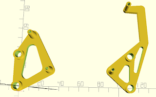
As I like the old style interface, I made up a cable to connect the two boards in that way... which led to the hiccup.  Whilst I had left enough space between my mount adapter and the SKR Mini to connect everything else, I hadn't left enough space above the screen connector on the controller, which was now a problem since I was going to use it after all..  A re-design of the the mount adapter was required, and I took this opportunity to split it into two parts.  On reflection, it seemed unnecessary to use a single part when there were two pairs of mounting points and leaving the left and right sides of the adapter completely separate would leave more space for not just the cabling but also some more airflow.  Maybe.  I didn't take a photo of the new arrangement, but here's a screen shot of the design.  Note the dog-leg on the right hand side.  The connector for the screen is directly below the board mount pillar at the top-right, so the frame has to do this to avoid blocking the socket.

Temperature sensing - using an 'unknown' Thermistor

A few years ago, I managed to break the thermistor which was used to monitor the temperature of the heated bed of my RepRap Mendel 3d Printer.  I didn't have a suitable replacement handy, so I substituted one that I had lying around, which made the controller think the bed was hotter than it was.  To compensate, I simply set the bed temperature to 50-100°C in 5° steps and measured the actual temperature of the surface.  Then I made a calibration graph so I could set the bed temperature in the slicing software such that the actual temperature would be what I wanted.  A horrific bodgy workaround, but it kept me printing until I could fix it properly.  The only thing I know about the thermistor I used is that its resistance is nominally 4700Ω at 25°C.

More recently, I've upgraded the controller and this seemed like a good opportunity to figure out how to make it work properly with the 'unknown' thermistor fitted.  What, you say? you're not going to just buy the proper thermistor, or at least one of those that Marlin already knows about, and fit that instead.  Of course not, that would be too easy.  I was going to do some science instead.

I'm still a little uncertain as to what exactly Marlin does to to translate thermistor resistance into temperature - does it create a lookup table from the values given when it starts up, or always calculate on the fly?  If you give it a look-up table as well as β and R25, does it always use the lookup table and ignore the given parameters?  I still don't know, but doesn't matter for the purpose of this exercise.

Thermistor Types & Marlin

There's a pretty good Wikipedia article about thermistors, which I encourage you to read if you know nothing about thermistors.  Marlin uses the Beta parameter equation mentioned there, and expects a NTC thermistor (i.e. one whose resistance decreases with temperature).  So we need to find the correct value of β, and a resistance at a known temperature and make those known to Marlin.  As with everything else configurable about Marlin, this is done by setting variables in configuration.h and configuration_adv.h before compiling the firmware from source.  I won't go into the details of that here, as there are plenty of good tutorials out there already.  I will just say that you need to specify a thermistor type for the heated bed in configuration.h - type number 1000 is conventionally used for custom thermistors, so find the line that begins 

    #define TEMP_SENSOR_BED 

and set it to read:

    #define TEMP_SENSOR_BED 1000

then change the values of β and R0 for thermistor type 1000 in configuration_adv.h:  find the section that begins

    #if TEMP_SENSOR_BED == 1000

and set it to read like this (substituting the values determined for β and resistance at 25°C)

    #if TEMP_SENSOR_BED == 1000
      #define BED_PULLUP_RESISTOR_OHMS     4700    // Pullup resistor
      #define BED_RESISTANCE_25C_OHMS      4675  // Resistance at 25C
      #define BED_BETA                     3885    // Beta value
    #endif

The Maths Bit

The equation we need is this one

 (1)

RT is resistance at temperature T

R0 is resistance at temperature T0

T is temperature

T0 is an arbitrary fixed temperature, we'll use the lowest temperature at which we measured the thermistor's resistance.

All temperatures are absolute, i.e. in Kelvin

If we take the natural logs of both sides of that, we get

  (2)

And so if we measure values of resistance and temperature and plot ln(RT) on the y axis against (1/T-1/T0) on the x axis, we should get a straight line with a gradient of β.

The Science bit

Method

A thermistor was immersed in near-boiling water and its resistance was monitored as it and the water cooled.  A digital thermometer with a remote probe was used for the temperature measurements, a digital multimeter for the resistance measurements.  The thermistor was kept close to the thermometer probe and the water stirred to keep the temperature difference between them as small as possible.  A graph of ln(RT) vs (1/T-1/T0) was plotted using a spreadsheet program and β determined using the spreadsheet's line of best fit function.  The resistance at 25°C was calculated using the value of β determined and equation (1).  Marlin firmware was then compiled using those two values for the heated bed thermistor, and installed onto a 3d printer controller.  The thermistor was connected to that controller and immersed once again into a vessel of hot water, alongside the same thermometer probe as before.  The temperatures reported by both the conroller board and the thermometer  were compared as the water cooled.

Results

A spreadsheet containing the results can be downloaded from here.  Here is the graph used to determine β - it's the 3885.1 in the formula for the line of best fit.  The spreadsheet function SLOPE was used to get the gradient, which was then used to calculate resistance at 25°C and other temperatures.

That's a pretty good straight line in my book.  I didn't write down the comparison of the controller board's measurements with the thermometer's measurements, but did note that the thermometer was around a degree higher at 85°C, falling to half a degree higher at 65°C then drifting out to be one degree higher again at 40°C.  Given that, in use there will be enough of a thermal barrier between the bed heater, the thermistor and the bed surface to produce a bigger discrepancy than that, I think that's a useable result.  So I'm going to use it.

A simpler alternative

The RepRap.org wiki shows a simpler method of doing this, using only two measurements.  The maths on that page is a little hard to follow, at least with the two browsers I've used to look at it (Chrome & Edge) because neither of them seems to understand the <math> tags.  Still, there's a little spreadsheet there which will calculate your β and R25.for you.  Let's have a quick look at the formula used for that.

β=LN(B5/B2) / ((1/(B6+273.15)) - (1/(B3+273.15)))

B5 contains R at the higher temperature, B2 contains R at the lower temperature.

Ln(B5/B2) is the same as LN(B5)-LN(B2) .... which is just the difference in y values of two points on the above graph.

B6 & B3 contain the temperatures (in Celsius) at which the resistances were measured.  Adding 273.15 turns them into Kelvin.  So the rest of that formula is the difference in x values of two points on the above graph.   So the formula boils down to (increase in y)/(increase in x) for two points on the graph - which is the definition of the gradient, which is  β. The two methods are therefore essentially the same, the simpler one using two points, the more thorough one using a larger set of data.  Using a larger set of data can reveal and compensate for errors of measurement.  More errors = not such a good straight line, using a line of best fit averages out random errors.  You have no chance of doing that with only two data points.  Still, if you have justifiable confidence in your measurements, the two-point method will work just fine.

Yet More 3D Printer Modifications

New Z-axis Lead Screws

Another thing I was never happy about with the Copymaster 300 was the z-axis lead screws.  As supplied, these were 4-start 2mm pitch screws, giving a lead (i.e. length of travel per revolution) of 8mm.  This is far too coarse for a z-axis in my view.  The z-axis does not need to move quickly, a few mm per second (i.e. <=10) is more than enough.  What it does need to do is move precisely and repeatably, ideally with a resolution of 10 microns or better.  It also needs to stay where it is when the motors are not energised, and that was the big problem I experienced:  with the x-carriage at or near the home position, the weight of the two stepper motors (x-axis & extruder), plus hot end plus the carriage itself plus the gantry was enough to rotate the z-axis and allow that end of the gantry to fall by a significant fraction of a millimetre when the motor current was turned off.  Usually.  This meant levelling the gantry again every time the printer was used, which was a tedious chore.  I decided to change the lead screws to something with a finer pitch.

First, I ordered some single start 1mm pitch lead screws and nuts from China.  They managed to send me the right nuts, but the wrong lead screws.  The screws turned out to be a 2-start 2mm pitch thread (i.e. 4mm lead per revolution).  That would probably have worked, but, not having any nuts to go with them, I decided to hedge my bets and order another pair of 1mm lead screws from another supplier, and some 2mm, 2-start nuts to go with the wrong lead screws.  I was bound to get something that would work, I hoped.  I can always use the leftovers for something else.  Don't yet know what, stay tuned.

In the meantime, I went to my local screwfix and bought a couple of lengths of M8 threaded rod, which has a pitch of 1.25mm, and made some anti-backlash nuts using standard M8 nuts, springs and some printed parts.  That actually worked really well, and I should probably have done it that way in the first place.   I've now got the 1mm lead screws I intended to use, and made another pair of anti-backlash nuts to go with them.

Here's the OpenSCAD design for the anti-backlash system.  two of the lead screw nuts were modified slightly to make this work:  two of their fixing holes were cut into slots so that they would engage the two lugs visible at the top of this part, preventing them from rotating with the lead screw whilst allowing the small vertical movement needed to allow the spring to push them against the thread.

Here's the finished item in-situ.  Next time I might make it so you can see the spring inside.

  

More 3d Printer Modifications

New controller for the Copymaster.

At the end of last year, the controller in my Copymaster 300 decided to kill itself by the classic method of having a dodgy ground connection, which then led to a ground loop in the USB link to the raspberry Pi which was controlling it via OctoPi.  This killed the USB-serial adapter on the board, and also the USB ports on the Pi.  The rest of the Pi still worked, including WiFi, and it's now relegated to controlling some LED pixels instead.  Don't need a USB port for that.  So a new controller board had to be found & installed.  After a bit of browsing the internet and watching YouTube videos (I recommend this Aussie chap who goes by the handle of  'teaching tech' for good instruction in all things 3D printing.

My research led me to conclude that there was really no point in trying to replace the board with another just like it or anything based on an 8-bit microcontroller when much more capable 32-bit controllers were readily available and not very expensive. Especially if you're willing to take a punt and order one direct from China via Aliexpress or Banggood or any of the other online outlets.  I chose the BigTreeTech SKR V1.3 controller and a set of TMC2208 stepper drivers plus a TFT24 display.  You can get these from via Aliexpress from BigTreeTech's 'store', which reduces the possibility of ending up with a fake. 

I won't go into detail about the process of setting the thing up and compiling the firmware (Marlin V2.something), as it's much better covered in Teaching Tech's own video on the subject.

I will mention that, perhaps obviously, neither the board itself nor the screen would fit neatly into the spaces of their predecessors, the mounting screw holes are in the wrong place.  I anticipated this, and but was confident that I could come up with something, made on my other 3d printer, that I could mount the new boards on and then mount that where the old ones were.  Turned out I was right.  I had to leave a USB cable plugged into the controller and dangle the other end outside, but I expected that too - not much chance of a completely different board having any of the connectors in the right place for the case panel cut-outs.

Here's the design for the controller board adapter.  The four larger diameter holes fit over the mounting pillars for the original board.  The one on the bottom right is taller because that also functions as a mouting pillar for the new board, along with the three smaller diameter pillars.

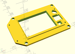
Here's the display board adapter.  The TFT24 is smaller than the original display, and both the screen and the encoder will fit inside the area of the original.  The part that stands proud of the main structure fits inside the panel cut-out for the old screen, with the new screen inside that.  The smaller square hole is for the reset switch, the larger one for the encoder body (the shaft just misses the edge of the raised area).  The circular hole is for the beeper.  Once again, the four large holes fit over the original mounts and the smaller ones are for the mounting screws for the new board.  The TFT 24 goes in there face up.

OctoPi

Still with the Raspberry Pi theme, for the last year or so I have been using Octopi to control both of my 3d printers.  Octopi is the Raspberry Pi version of Octoprint, which allows a host computer to send instructions to and receive telemetry from a 3d printer.  This is done through a web-based user interface, i.e. any device running a web browser on the same network as the printer can can simply navigate to 'http://<host name of computer running Octoprint>.local'  or 'http://<ip address of computer running Octoprint>' and see an interactive web page which will let them control the printer and monitor its progress.  If the Octoprint host has a webcam, that can be used to make time-lapse movies of the printing process.

For more details, see https://octoprint.org/

The two controlling my 3d printers connect to my wifi network, which works just fine whilst they're at home, if they were to be taken elsewhere then they'd need to be reconfigured to work on their own or on some other network.  Recently, I built a system for a friend which used the same trick as the mustard tin music players and the lightwand - provide an access point with DNS and DHCP servers so that a browser-equipped device can connect to it's little network and provide a user interface just about anywhere.

See https://thepi.io/how-to-use-your-raspberry-pi-as-a-wireless-access-point/  for a guide on how to set up an access point.

Shutting Down A Raspberry Pi

You can probably tell from the other posts in this blog that I'm a big fan of the Raspberry Pi microcomputer and have used it for several of my projects, usually without such niceties as a keyboard, mouse or monitor.  Using it in this way raises the issue of how to shut it down nicely so as not to avoid corrupting its boot disc (i.e. the SD card) by switching off the power suddenly.  My standard approach to this is to use a gpio pin to look for a signal to shut down the system.  I also find it useful, or at least comforting, to use another gpio pin to make an LED flash to indicate that the Pi is running and another one to light another LED to indicate that shutting-down is in progress.

When the Pi starts up, it runs a Python program called 'ShutdownCheck.py'.

ShutdownCheck.py assigns two gpio pins to be outputs, one for a red LED, one for a green LED, plus a 3rd gpio pin as an input.  The input pin is pulled high by the SoC's internal pull-up resistor, and can be pulled low by connecting it to ground through a simple momentary action switch, such as the type found in obsolete mice an on the front panels of outdated PCs that you found in a skip.  The LEDs' anodes are connected to output pins, their cathodes through a common resistor to ground  ShutdownCheck.py toggles the state of the output pin with the green LED and checks the input pin.  If the input pin is still high, it goes to sleep for a few seconds before looping back to toggle the green LED and check the input pin again.  If the input pin has gone low, i.e. the switch has been actuated, then the program sets the red LED's output pin high, sets the green LED's pin low and issues the command 'sudo shutdown -h now' - which will shut down the system.

A small variation on this, which I used recently because I had some 3-colour common-cathode LEDs, was to have the green & blue LEDs light up alternately until the shutdown request is received.  The python code for that version is shown below. 

# Python Script to check for shutdown request, alternate blue
# and green LEDs when running and light a red LED when shutting 
# down.  When red LED goes out again, Pi can be powered-off.
# Works well with a common-cathode RGB LRD.

import RPi.GPIO as GPIO
from os import system
from time import sleep

# set up GPIO pins to check for shutdown request
# and to light up LEDs.  Alternating Green/blue LEDs when active
# red LED during shutdown.  Note sdcheck is active
# low, i.e. grounded through switch to shut down.

sdcheck = 26
redled = 19
grnled = 13
bluled = 6

GPIO.setmode(GPIO.BCM)
GPIO.setup(redled,GPIO.OUT)
GPIO.setup(grnled,GPIO.OUT)
GPIO.setup(bluled,GPIO.OUT)
GPIO.setup(sdcheck,GPIO.IN, pull_up_down=GPIO.PUD_UP)

green_on = 1
blue_on = 0

while True:
	green_on = (green_on+1) % 2
	blue_on = (blue_on+1) % 2
	GPIO.output (grnled,green_on)
	GPIO.output (bluled,blue_on)
	if not (GPIO.input(sdcheck)):
	  print("Shutdown request received")
	  GPIO.output(grnled,GPIO.LOW)
	  GPIO.output(bluled,GPIO.LOW)
	  GPIO.output(redled,GPIO.HIGH)
	  system("sudo shutdown -h now")
	  break
	sleep(5)

I inverted the logic of the shutdown request (i.e. low input, not high, is interpreted as the command to shut down) as it does not need to use any of the powered pins that would be necessary for the 'normal' protocol, just the gpio pins and ground.

I've settled on using the four (or five for the r,g,b version) pins at the bottom left corner of the gpio header, as seen with the USB ports at the bottom and the gpio header on the right, as shown in the illustration right. Below is a photo of a switch plus red & green LEDs built onto a small header plug.